The High Performance Scripting team at Intel Labs recently released ParallelAccelerator.jl, a Julia package for high-performance, high-level array-style programming. The goal of ParallelAccelerator is to make high-level array-style programs run as efficiently as possible in Julia, with a minimum of extra effort required from the programmer. In this post, we'll take a look at the ParallelAccelerator package and walk through some examples of how to use it to speed up some typical array-style programs in Julia.
Introduction
Ideally, high-level array-style Julia programs should run as efficiently as possible on high-performance parallel hardware, with a minimum of extra programmer effort required, and with performance reasonably close to that of an expert implementation in C or C++. There are three main things that ParallelAccelerator does to move us toward this goal:
First, we identify implicit parallel patterns in array-style code the user writes. We'll say more about these parallel patterns shortly.
Second, we compile these parallel patterns to explicit parallel loops.
Third, we minimize runtime overheads incurred by things like array bounds checks and intermediate array allocations.
The key user-facing feature that the ParallelAccelerator package provides is a Julia macro called @acc, which is short for "accelerate". Annotating functions or blocks of code with @acc lets you designate the parts of your Julia program that you want to compile to optimized native code. Here's a toy example of using @acc to annotate a function:
julia> using ParallelAccelerator

julia> @acc f(x) = x .+ x .* x
f (generic function with 1 method)

julia> f([1,2,3,4,5])
5-element Array{Int64,1}:
2
6
12
20
30
Under the hood, ParallelAccelerator is essentially a compiler – itself implemented in Julia – that intercepts the usual Julia JIT compilation process for @acc-annotated functions. It compiles @acc-annotated code to C++ OpenMP code, which can then be compiled to a native library by an external C++ compiler such as GCC or ICC. (This intermediate C++ generation step isn't essential to the design of ParallelAccelerator, though – instead, the compiler could target Julia's own forthcoming native threading backend. [1]) On the Julia side, ParallelAccelerator generates a proxy function that calls into that native library, and replaces calls to @acc-annotated functions, like f in the above example, with calls to the appropriate proxy function.
We'll say more shortly about the parallel patterns that ParallelAccelerator targets and about how the ParallelAccelerator compiler works, but before we do, let's look at some code and some performance results.
A quick preview of results: Black-Scholes option pricing benchmark
Let's see how to use ParallelAccelerator to speed up a classic high-performance computing benchmark: an implementation of the Black-Scholes formula for option pricing. The following code is a Julia implementation of the Black-Scholes formula.
function cndf2(in::Array{Float64,1})
    out = 0.5 .+ 0.5 .* erf(0.707106781 .* in)
    return out
end

function blackscholes(sptprice::Array{Float64,1},
                      strike::Array{Float64,1},
                      rate::Array{Float64,1},
                      volatility::Array{Float64,1},
                      time::Array{Float64,1})
    logterm = log10(sptprice ./ strike)
    powterm = .5 .* volatility .* volatility
    den = volatility .* sqrt(time)
    d1 = (((rate .+ powterm) .* time) .+ logterm) ./ den
    d2 = d1 .- den
    NofXd1 = cndf2(d1)
    NofXd2 = cndf2(d2)
    futureValue = strike .* exp(- rate .* time)
    c1 = futureValue .* NofXd2
    call = sptprice .* NofXd1 .- c1
    put  = call .- futureValue .+ sptprice
end

function run(iterations)
    sptprice   = Float64[ 42.0 for i = 1:iterations ]
    initStrike = Float64[ 40.0 + (i / iterations) for i = 1:iterations ]
    rate       = Float64[ 0.5 for i = 1:iterations ]
    volatility = Float64[ 0.2 for i = 1:iterations ]
    time       = Float64[ 0.5 for i = 1:iterations ]

    tic()
    put = blackscholes(sptprice, initStrike, rate, volatility, time)
    t = toq()
    println("checksum: ", sum(put))
    return t
end
Here, the blackscholes function takes five arguments, each of which is an array of Float64s. The run function initializes these five arrays and passes them to blackscholes, which, along with the cndf2 (cumulative normal distribution) function that it calls, does several computations involving pointwise addition (.+), subtraction (.-), multiplication (.*), and division (./) on the arrays. It's not necessary to understand the details of the Black-Scholes formula; the important thing to notice about the code is that we are doing lots of pointwise array arithmetic. Using Julia 0.4.4-pre on a 4-core Ubuntu 14.04 desktop machine with 8 GB of memory, the run function takes about 11 seconds to run when called with an argument of 40,000,000 (meaning that we are dealing with 40-million-element arrays):
julia> @time run(40_000_000)
checksum: 8.381928525856283e8
 12.885293 seconds (458.51 k allocations: 9.855 GB, 2.95% gc time)
11.297714183
Here, the 11.297714183 being returned from run is the number of seconds it takes the blackscholes call alone to return. The 12.885293 seconds reported by @time is a little longer, because it's the running time of the entire run call.
The many pointwise array operations in this code make it a great candidate for speeding up with ParallelAccelerator (as we'll discuss more shortly). Doing so requires only minor changes to the code: we import the ParallelAccelerator library with using
ParallelAccelerator, then wrap the cndf2 and blackscholes functions in an @acc block, as follows:
using
ParallelAccelerator
@acc begin
function cndf2(in::Array{Float64,1})
out = 0.5 .+ 0.5 .* erf(0.707106781 .* in)
return out
end
function blackscholes(sptprice::Array{Float64,1},
strike::Array{Float64,1},
rate::Array{Float64,1},
volatility::Array{Float64,1},
time::Array{Float64,1})
logterm = log10(sptprice ./ strike)
powterm = .5 .* volatility .* volatility
den = volatility .* sqrt(time)
d1 = (((rate .+ powterm) .* time) .+ logterm) ./ den
d2 = d1 .- den
NofXd1 = cndf2(d1)
NofXd2 = cndf2(d2)
futureValue = strike .* exp(- rate .* time)
c1 = futureValue .* NofXd2
call = sptprice .* NofXd1 .- c1
put = call .- futureValue .+ sptprice
end
endThe definition of run stays the same. With the addition of the @acc wrapper, we now have much better performance:
julia> @time run(40_000_000)
checksum: 8.381928525856283e8
  4.010668 seconds (1.90 M allocations: 1.584 GB, 2.06% gc time)
3.503281464
This time, blackscholes returns in about 3.5 seconds, and the entire run call finishes in about 4 seconds. This is already an improvement, but on subsequent calls to run, we do even better:
julia> @time run(40_000_000)
checksum: 8.381928525856283e8
  1.418709 seconds (158 allocations: 1.490 GB, 8.98% gc time)
1.007861068

julia> @time run(40_000_000)
checksum: 8.381928525856283e8
  1.410865 seconds (154 allocations: 1.490 GB, 7.93% gc time)
1.012813958
In subsequent calls, run finishes in about a second, with the entire call taking about 1.4 seconds. The reason for this additional improvement is that ParallelAccelerator has already compiled the blackscholes and cndf2 functions and doesn't need to do so again on subsequent runs.
These results were collected on an ordinary desktop machine, but we can scale up further. The following figure reports the time it takes blackscholes to run on arrays of 100 million elements, this time on a 36-core machine with 128 GB of RAM [2]:
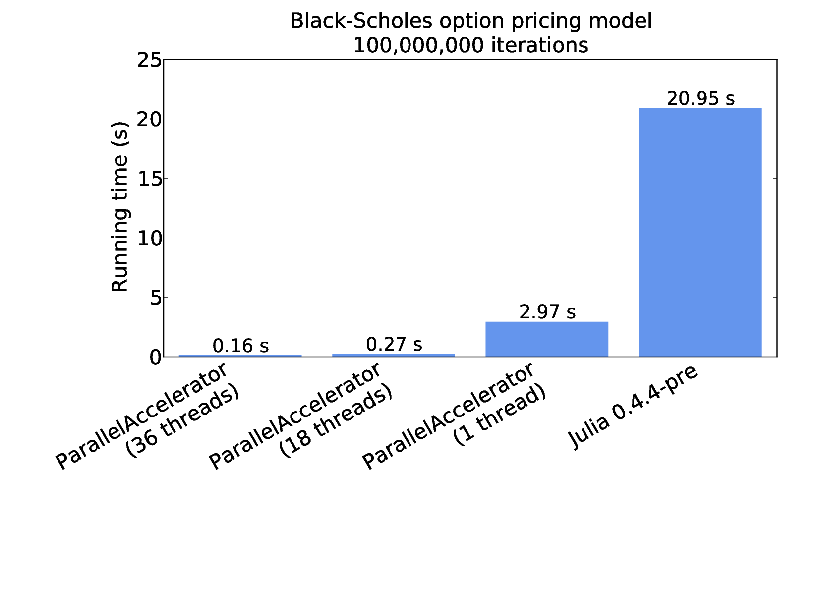
The first three bars of the above figure show performance results for ParallelAccelerator using different numbers of threads. Since ParallelAccelerator compiles Julia to OpenMP C++, we can use the OMP_NUM_THREADS environment variable to control the number of threads that the code runs with. Here, with OMP_NUM_THREADS set to 18, blackscholes runs in 0.27 seconds; with 36 threads (matching the number of cores on the machine), running time drops to 0.16 seconds. The third bar shows results for ParallelAccelerator with OMP_NUM_THREADS set to 1, which clocks in at about 3 seconds. For comparison, the rightmost bar show results for "plain Julia", that is, a version of the code without @acc, which runs in about 21 seconds.
Because Julia doesn't (yet) have native multithreading support, the plain Julia results shown in the rightmost bar are for one thread. But it is interesting to note that the ParallelAccelerator implementation of Black-Scholes outperforms plain Julia by a factor of about seven, even when running on just one core. The reason for this speedup is that ParallelAccelerator (despite its name!) does more than just parallelize code. The ParallelAccelerator compiler is able to do away with much of the runtime overhead incurred by array bounds checks and allocation of intermediate arrays. After that, with the addition of parallelism, we're able to do even better, for a total speedup of more than 100x over plain Julia.
To see how ParallelAccelerator accomplishes this, we'll discuss the parallel patterns that ParallelAccelerator handles in a bit more detail, and then we'll take a closer look at the ParallelAccelerator compiler pipeline.
Parallel patterns
ParallelAccelerator works by identifying implicit parallel patterns in source code and making the parallelism explicit. These patterns include map, reduce, array comprehension, and stencil.
Map
As we saw in the Black-Scholes example above, the .+, .-, .*, and ./ operations in Julia are pointwise array operations that take input arrays as arguments and produce an output array. ParallelAccelerator translates these pointwise array operations into data-parallel map operations. (See the ParallelAccelerator documentation for a complete list of all the pointwise array operations that it knows how to parallelize.) Furthermore, ParallelAccelerator translates array assignments into in-place map operations. For instance, assigning a = a .* b where a and b are arrays would map .* over a and b and update a in place with the result. For both standard map and in-place map, it is possible for ParallelAccelerator to avoid any array bounds checking once we've established that the input arrays and the output arrays are the same size.
Reduce
Reduce operations take an array argument and produce a scalar result by combining all the elements of an array with an associative and commutative operation. ParallelAccelerator translates the Julia functions minimum, maximum, sum, prod, any, and all into data-parallel reduce operations when they are called on arrays.
Array comprehension
Julia supports array comprehensions, a convenient and concise way to construct arrays. For example, the expressions that initialize the five input arrays in the Black-Scholes example above are all array comprehensions. As a more sophisticated example, the following avg function, taken from the Julia manual, takes a one-dimensional input array x of length n and uses an array comprehension to construct an output array of length n-2, in which each element is a weighted average of the corresponding element in the original array and its two neighbors:
avg(x) = [ 0.25*x[i-1] + 0.5*x[i] + 0.25*x[i+1] for i = 2:length(x) - 1 ]Comprehensions like this one can also be parallelized by ParallelAccelerator: in a nutshell, ParallelAccelerator can transform array comprehensions to code that first allocates an output array and then performs an in-place map that can write to each element of the output array in parallel.
Array comprehensions differ from map and reduce operations in that they involve explicit array indexing. But it is still possible to parallelize array comprehensions in Julia, as long as there are no side effects in the comprehension body (everything before the for). [3] ParallelAccelerator uses a conservative static analysis to try to identify and reject side-effecting operations in comprehensions.
Stencil
In addition to map, reduce, and comprehension, ParallelAccelerator targets a fourth parallel pattern: stencil computations. A stencil computation updates the elements of an array according to a fixed pattern called a stencil. In fact, the avg comprehension example above could also be thought of as a stencil computation, because it updates the contents of an array based on each element's neighbors. However, stencil computations differ from the other patterns that ParallelAccelerator targets, because there's not a built-in, user-facing language feature in Julia that expresses stencil computations specifically. So, ParallelAccelerator introduces a new user-facing language construct called runStencil for expressing stencil computations in Julia. Next, we'll look at an example that illustrates how runStencil works.
Example: Blurring an image with runStencil
Let's consider a stencil computation that blurs an image using a Gaussian blur. The image is represented as a two-dimensional array of pixels. To blur the image, we set the value of each output pixel to a particular weighted average of the corresponding input pixel's value and the values of its neighboring input pixels. By repeating this process multiple times, we can get an increasingly blurred image. [4]
The following code implements a Gaussian blur in Julia. It operates on a 2D array of Float32s: the pixels of the source image. It's easy to obtain such an array using, for instance, the load function from the Images.jl library, followed by a call to convert to get an array of type Array{Float32,2}. (For simplicity, we're assuming that the input image is a grayscale image, so each pixel has just one value instead of red, green, and blue values. However, it would be straightforward to use the same approach for RGB pixels.)
function blur(img::Array{Float32,2}, iterations::Int)
    w, h = size(img)
    for i = 1:iterations
      img[3:w-2,3:h-2] =
           img[3-2:w-4,3-2:h-4] * 0.0030 + img[3-1:w-3,3-2:h-4] * 0.0133 + img[3:w-2,3-2:h-4] * 0.0219 + img[3+1:w-1,3-2:h-4] * 0.0133 + img[3+2:w,3-2:h-4] * 0.0030 +
           img[3-2:w-4,3-1:h-3] * 0.0133 + img[3-1:w-3,3-1:h-3] * 0.0596 + img[3:w-2,3-1:h-3] * 0.0983 + img[3+1:w-1,3-1:h-3] * 0.0596 + img[3+2:w,3-1:h-3] * 0.0133 +
           img[3-2:w-4,3+0:h-2] * 0.0219 + img[3-1:w-3,3+0:h-2] * 0.0983 + img[3:w-2,3+0:h-2] * 0.1621 + img[3+1:w-1,3+0:h-2] * 0.0983 + img[3+2:w,3+0:h-2] * 0.0219 +
           img[3-2:w-4,3+1:h-1] * 0.0133 + img[3-1:w-3,3+1:h-1] * 0.0596 + img[3:w-2,3+1:h-1] * 0.0983 + img[3+1:w-1,3+1:h-1] * 0.0596 + img[3+2:w,3+1:h-1] * 0.0133 +
           img[3-2:w-4,3+2:h-0] * 0.0030 + img[3-1:w-3,3+2:h-0] * 0.0133 + img[3:w-2,3+2:h-0] * 0.0219 + img[3+1:w-1,3+2:h-0] * 0.0133 + img[3+2:w,3+2:h-0] * 0.0030
    end
    return img
end
Here, to compute the value of a pixel in the output image, we use the the corresponding input pixel as well as all its neighboring pixels, to a depth of two pixels out from the input pixel – so, twenty-four neighbors. In all, there are twenty-five pixel values to examine. We add all these pixel values together, each multiplied by a weight – in this case 0.0030 for the cornermost pixels, 0.1621 for the center pixel, and for all the other pixels, something in between – and the total is the value of the output pixel. At the borders of the image, we don't have enough neighboring pixels to compute an output pixel value, so we simply skip those pixels and don't assign to them. [5]
Notice that the blur function explicitly loops over the number of iterations, that is, times to apply the blur to the the image, but it does not explicitly loop over pixels in the image. Instead, the code is written in array style: it performs just one assignment to the array img, using the ranges 3:w-2 and 3:h-2 to avoid assigning to the borders of the image. On a large grayscale input image of 7095 by 5322 pixels, this code takes about 10 minutes to run for 100 iterations.
Using ParallelAccelerator, we can get much better performance. Let's look at a version of blur that uses runStencil:
@acc function blur(img::Array{Float32,2}, iterations::Int)
    buf = Array(Float32, size(img)...)
    runStencil(buf, img, iterations, :oob_skip) do b, a
       b[0,0] =
            (a[-2,-2] * 0.003  + a[-1,-2] * 0.0133 + a[0,-2] * 0.0219 + a[1,-2] * 0.0133 + a[2,-2] * 0.0030 +
             a[-2,-1] * 0.0133 + a[-1,-1] * 0.0596 + a[0,-1] * 0.0983 + a[1,-1] * 0.0596 + a[2,-1] * 0.0133 +
             a[-2, 0] * 0.0219 + a[-1, 0] * 0.0983 + a[0, 0] * 0.1621 + a[1, 0] * 0.0983 + a[2, 0] * 0.0219 +
             a[-2, 1] * 0.0133 + a[-1, 1] * 0.0596 + a[0, 1] * 0.0983 + a[1, 1] * 0.0596 + a[2, 1] * 0.0133 +
             a[-2, 2] * 0.003  + a[-1, 2] * 0.0133 + a[0, 2] * 0.0219 + a[1, 2] * 0.0133 + a[2, 2] * 0.0030)
       return a, b
    end
    return img
end
Here, we again have a function called blur – now annotated with @acc – that takes the same arguments as the original code. This version of blur allocates a new 2D array called buf that is the same size as the original img array. The allocation of buf is followed by a call to runStencil. Let's take a closer look at the runStencil call.
runStencil has the following signature:
runStencil(kernel :: Function, buffer1, buffer2, ..., iteration :: Int, boundaryHandling :: Symbol)In blur, the call to runStencil uses Julia's do-block syntax for function arguments, so the do b, a ... end block is actually the first argument to the runStencil call. The do block creates an anonymous function that binds the variables b and a. The arguments buffer1, buffer2,
... that are passed to runStencil become the arguments to the anonymous function. In this case, we are passing two buffers, buf and img, to runStencil, and so the anonymous function takes two arguments.
Aside from the anonymous function and the two buffers, runStencil takes two other arguments. The first of these is a number of iterations that we want to run the stencil computation for. In this case, we simply pass along the iterations argument that is passed to blur. Finally, the last argument to runStencil is a symbol indicating how stencil boundaries are to be handled. Here, we're using the :oob_skip symbol, short for "out-of-bounds skip". It means that when input indices are out of bounds – for instance, in the situation where the input pixel is one of those on the two-pixel border of the image, and there aren't enough neighbor pixels to compute the output pixel value – then we simply skip writing to the output pixel. This has the same effect as the careful indexing in the original version of blur.
Finally, let's look at the body of the do block that we're passing to runStencil. It contains an assignment to b, using values computed from a. As we've said, b and a here are buf and img: our newly-allocated buffer, and the original image. The code here is similar to that of the original implementation of blur, but here we're using relative rather than absolute indexing into arrays, The index 0,0 in b[0,0] doesn't refer to any particular element of b, but instead to the current position of a cursor that can be thought of as traversing all the elements of b. On the right side of the assignment. a[-2,-1] refers to the element in a that is two elements to the left and one element up from the 0,0 element of a. In this way, we can express a stencil computation more concisely than the original version of blur did, and we don't have to worry about getting the indices correct for boundary handling as we had to do before, because the :oob_skip argument tells runStencil everything it needs to no to handle boundaries correctly.
Finally, at the end of the do block, we return a, b. They were bound as b, a, but we return them in the opposite order so that for each iteration of the stencil, we'll be using the already-blurred buffer as the input for another round of blurring. This continues for however many iterations we've specified. There's therefore no need to write an explicit for loop for stencil iterations when using runStencil; one just passes an argument saying how many iterations should occur.
Therefore runStencil enables us to write more concise code than plain Julia, as we'd expect from a language extension. But where runStencil really shines is in the performance it enables. The following figure compares performance results for plain Julia and ParallelAccelerator implementations of blur, each running for 100 iterations on the aforementioned 7095x5322 source image, run using the same machine as for the previous Black-Scholes benchmark.
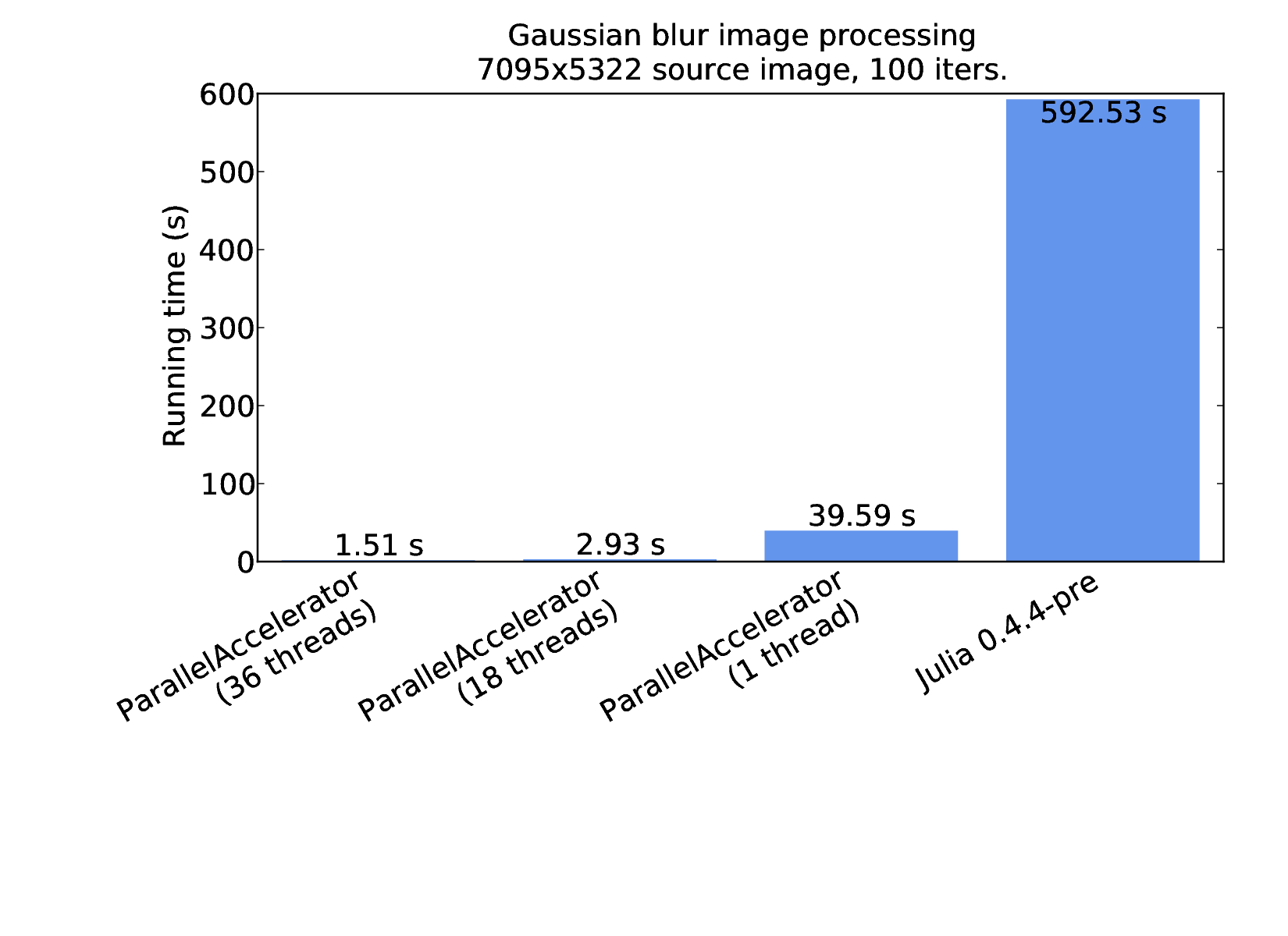
The rightmost column shows the results for plain Julia, using the first implementation of blur shown above. The three columns to the left show results for the ParallelAccelerator version that uses runStencil. As we can see, even when running on just one thread, ParallelAccelerator enables a speedup of about 15x: from about 600 seconds to about 40 seconds. Running on 36 threads provides a further parallel speedup of more than 26x, resulting in a total speedup of nearly 400x over plain single-threaded Julia.
An overview of the ParallelAccelerator compiler architecture
Now that we've talked about the parallel patterns that ParallelAccelerator speeds up and seen some code examples, let's take a look at how the ParallelAccelerator compiler works.
The standard Julia JIT compiler parses Julia source code into the Julia abstract syntax tree (AST) representation. It performs type inference on the AST, then transforms the AST to LLVM IR, and finally generates native assembly code. ParallelAccelerator intercepts this process at the level of the AST. It introduces new AST nodes for the parallel patterns we discussed above. It then does various optimizations on the resulting AST. Finally, it generates C++ code that can be compiled by an external C++ compiler. The following figure shows an overview of the ParallelAccelerator compilation process:
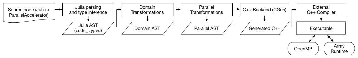
As many readers of this blog will know, Julia has good support for inspecting and manipulating its own ASTs. Its built-in code_typed function will return the AST of any function after Julia's type inference has taken place. This is very convenient for ParallelAccelerator, which is able to use the output from code_typed as the input to the first pass of its compiler, which is called "Domain Transformations". The Domain Transformations pass produces ParallelAccelerator's Domain AST intermediate representation.
Domain AST is similar to Julia's AST, except it introduces new AST nodes for parallel patterns that it identifies. We call these nodes "domain nodes", collectively. The Domain Transformations pass replaces certain parts of the AST with domain nodes.
The Domain Transformations pass is followed by the Parallel Transformations pass, which replaces domain nodes with "parfor" nodes, each of which represents one or more nested parallel for loops. Loop fusion also takes place during the Parallel Transformations pass. We call the result of Parallel Transformations Parallel AST. [6]
The compiler hands off Parallel AST code to the last pass of the compiler, CGen, which generates C++ code and converts parfor nodes into OpenMP loops. Finally, an external C++ compiler creates an executable which is linked to OpenMP and to a small array runtime component written in C that manages the transfer of arrays back and forth between Julia and C++.
Caveats
ParallelAccelerator is still a proof of concept at this stage. Users should be aware of two issues that can stand in the way of being able to make effective use of ParallelAccelerator. Those issues are, first, package load time, and second, limitations in what Julia programs ParallelAccelerator is able to handle. We discuss each of these issues in turn.
Package load time
Because ParallelAccelerator is a large Julia package (it's a compiler, after all), it takes a long time (perhaps 20 or 25 seconds on a 4-core desktop machine) for using ParallelAccelerator to run. This long pause is not the time that ParallelAccelerator is taking to compile your @acc-annotated code; it's the time that Julia is taking to compile ParallelAccelerator itself. After this initial pause, the first call to an @acc-annotated function will incur a brief compilation pause (this time from the ParallelAccelerator compiler, not Julia itself) of perhaps a couple of seconds. Subsequent calls to the same function won't incur the compilation pause.
Let's see what these compilation pauses look like in practice. The ParallelAccelerator package comes with a collection of example programs that print timing information, including the Black-Scholes and Gaussian blur examples shown in this post. All the examples print timing information for two calls to an @acc-annotated function: first a "warm-up" call with trivial arguments to measure compilation time, and then a more realistic call. In the output printed by each example, timing information for the more realistic call is preceded by the string "SELFTIMED", while timing information for the warm-up call is preceded by "SELFPRIMED". Let's run the Black-Scholes example and time it using the time shell command:
$ time julia ParallelAccelerator/examples/black-scholes/black-scholes.jl
iterations = 10000000
SELFPRIMED 1.766323497
checksum: 2.0954821257116848e8
rate = 1.9205394841503927e8 opts/sec
SELFTIMED 0.052068703

real	0m26.454s
user	0m31.027s
sys	0m0.874s
Here, we're running Black-Scholes for 10,000,000 iterations on our 4-core desktop machine. The total wall-clock time of 26.454 seconds consists mostly of the time it takes for using ParallelAccelerator to run. Once that's done, Julia reports a SELFPRIMED time of about 1.8 seconds, which is dominated by the time it takes for ParallelAccelerator to compile the @acc-annotated code, and finally the SELFTIMED time is about 0.05 seconds for this problem size.
As Julia's compilation speed improves, we expect that package load time will be less of a problem for ParallelAccelerator.
Compiler limitations
ParallelAccelerator is able to handle only a limited subset of Julia language features, and it only supports a limited subset of Julia's Base library functions. In other words, you cannot yet put an @acc annotation on arbitrary Julia code and expect it to go faster out of the box. The examples in this post give an idea of what kinds of programs are supported currently; for more, check out the full collection of ParallelAccelerator examples. However, if ParallelAccelerator can't compile some code in an @acc-annotated function, it will simply fall back to running the function under regular Julia. So your code will run, regardless of whether ParallelAccelerator can speed it up.
One reason why an @acc-annotated function might fail to compile is that ParallelAccelerator tries to transitively compile every Julia function that is called by the @acc-annotated function. So, if an @acc-annotated function makes several Julia library calls, ParallelAccelerator will attempt to compile those functions as well – and every Julia function that they call, and so on. If any of the code in the call chain contains a feature that ParallelAccelerator doesn't currently support, ParallelAccelerator will fail to compile the original @acc-annotated function. It is therefore a good idea to begin by annotating small (but expensive) computational kernels with @acc, rather than wrapping an entire program in an @acc block. The ParallelAccelerator documentation has many more details on which Julia features we don't support and why.
These limitations explain why the kind of performance improvements that ParallelAccelerator provides aren't already the default in Julia. Supporting all of Julia would be a major undertaking; however, in many cases, there's not a fundamental reason why ParallelAccelerator couldn't support a particular Julia feature or a function in Base, and supporting it is a matter of realizing that it is a problem for users and putting in the necessary engineering effort to fix it. So, when you come across code that ParallelAccelerator can't handle, please do file bugs!
Conclusion
In this post, we've introduced ParallelAccelerator.jl, a package for speeding up array-style Julia programs. It works by identifying implicit parallel patterns in source code and compiling them to efficient, explicitly parallel executables, along the way getting rid of many of the usual overheads of high-level array-style programming.
ParallelAccelerator is an open source project in its early stages, and we enthusiastically encourage comments, questions, bug reports, and contributions from the Julia community. We welcome everyone's participation, and we are especially interested in how ParallelAccelerator can be used to speed up real-world Julia programs.
[1] Starting with Julia 0.5, Julia will have its own native threading support, which means that ParallelAccelerator can target Julia's own native threads instead of generating C++ OpenMP code for parallelism. We've begun work on implementing a native-threading-based backend for ParallelAccelerator, but we still target C++ by default.
[2] Detailed machine and benchmarking specifications: We use a machine with two Intel Xeon E5-2699 v3 processors (2.3 GHz) with 18 physical cores each and 128 GB RAM, running the CentOS 6.7 Linux distribution. We use the Intel C++ Compiler (ICC) v15.0.2 with "-O3" for compilation of the generated C++ code. The Julia version is 0.4.4-pre+26. The results shown are the average of three runs (we run each version of a benchmark five times and discard the first and last runs).
[3] In Julia, it is not possible to index into a comprehension's output array in the body of the comprehension. (The avg example indexes only into the input array, not the output array.) Therefore, it's not necessary to do any bounds checking on writes to the output array. However, we still need to bounds-check reads from the input array (for instance, in the avg example, if we'd written 0.25*x[i-2], that would be out of bounds), so we cannot avoid all array bounds checking for comprehensions in the way that we can for map operations.
[4] In practice, rather than applying successive Gaussian blurs to an image, we'd probably apply a single, larger Gaussian blur, which, as Wikipedia notes, is at least as efficient computationally. Nevertheless, we'll use it here as an example of a stencil computation that can be iterated.
[5] A more sophisticated implementation of Gaussian blur might do a fancier form of border handling, using only the pixels it has available at the borders.
[6] The names "Domain AST" and "Parallel AST" are inspired by the Domain IR and Parallel IR of the Delite compiler framework.