Machine learning is a huge discipline, with applications ranging from natural language processing to solving partial differential equations. It is from this landscape that major frameworks such as PyTorch, TensorFlow, and Flux.jl arise and strive to be packages for "all of machine learning". While some of these frameworks have the backing of large companies such as Facebook and Google, the Julia community has relied on the speed and productivity of the Julia programming language itself in order for its open source community to keep up with the pace of development. It is from this aspect which Flux.jl derives its "slimness": while PyTorch and TensorFlow include entire separate languages and compilers (torchscript, XLA, etc.), Flux.jl is just Julia. It is from this that the moniker "you could have built it yourself" is commonly used to describe Flux.jl.
In this post we take a different look at how the programmability of Julia helps in the machine learning space. Specifically, by targeting the grand space of "all machine learning", frameworks inevitably make trade-offs that accelerate some aspects of the code to the detriment of others. This comes from the inevitable trade-off between simplicity, generality, and performance. However, the ability to easily construct machine learning libraries thus presents an interesting question: can this development feature be used to easily create alternative frameworks which focus its performance on more non-traditional applications or aspects?
The answer is yes, you can quickly build machine learning implementations which greatly outperform the frameworks in specialized cases using the Julia programming language, and we demonstrate this with our new package: SimpleChains.jl.
Scientific Machine Learning (SciML) and "Small" Neural Networks
SimpleChains.jl is a library developed by Pumas-AI and JuliaHub in collaboration with Roche and the University of Maryland, Baltimore. The purpose of SimpleChains.jl is to be as fast as possible for small neural networks. SimpleChains.jl originated as a solution for the Pumas-AI's DeepPumas product for scientific machine learning (SciML) in healthcare data analytics. As an illustration, small neural networks (and other approximators, such as Fourier series or Chebyshev polynomial expansions) can be combined with known semi-physiologic models to discover previously unknown mechanisms and prognostic factors. For a short introduction to how this is done, check out the following video by Niklas Korsbo:
This SciML methodology has been shown across many disciplines, from black hole dynamics to the development of earthquake safe buildings, to be a flexible method capable of discovering/guiding (bio)physical equations. Here's a recent talk which walks through the various use cases of SciML throughout the sciences:
For more details on the software and methods, see our paper on Universal Differential Equations for Scientific Machine Learning.
The unique aspects of how neural networks are used in these contexts make them rife for performance improvements through specialization. Specifically, in the context of machine learning, one normally relies on the following assumption: the neural networks are large enough that the O(n^3) cost of matrix-matrix multiplication (or other kernels like convolutions) dominates the the runtime. This is essentially the guiding principle behind most of the mechanics of a machine learning library:
Matrix-matrix multiplication scales cubicly while memory allocations scale linearly, so attempting to mutate vectors with non-allocating operations is not a high priority. Just use
A*x.Focus on accelerating GPU kernels to be as fast as possible! Since these large matrix-matrix operations will be fastest on GPUs and are the bottleneck, performance benchmarks will essentially just be a measurement of how fast these specific kernels are.
When doing reverse-mode automatic differentiation (backpropagation), feel free to copy values to memory. Memory allocations will be hidden by the larger kernel calls.
Also, feel free to write a "tape" for generating backpropagation. The tape does add the cost of essentially building a dictionary during the forward pass, but that will be hidden by the larger kernel calls.
Do these assumptions actually hold in our case? And if they don't, can we focus on these aspects to draw more performance out for our use cases?
Digging In: Small Neural Network Performance Overheads
It's easy to show that these assumptions breakdown when we start focusing on this smaller neural network use case. For starters, let's look at assumptions (1)(2). It's not hard to show where these two will unravel:
using LinearAlgebra, BenchmarkTools, CUDA, LoopVectorization

function mygemmturbo!(C, A, B)
    @tturbo for m ∈ axes(A, 1), n ∈ axes(B, 2)
        Cmn = zero(eltype(C))
        for k ∈ axes(A, 2)
            Cmn += A[m, k] * B[k, n]
        end
        C[m, n] = Cmn
    end
end

function alloc_timer(n)
    A = rand(Float32,n,n)
    B = rand(Float32,n,n)
    C = rand(Float32,n,n)
    t1 = @belapsed $A * $B
    t2 = @belapsed (mul!($C,$A,$B))
    t3 = @belapsed (mygemmturbo!($C,$A,$B))
    A,B,C = (cu(A), cu(B), cu(C))
    t4 = @belapsed CUDA.@sync($A * $B)
    t5 = @belapsed CUDA.@sync(mul!($C,$A,$B))
    t1,t2,t3,t4,t5
end
ns = 2 .^ (2:11)
res = [alloc_timer(n) for n in ns]
alloc      = [t[1] for t in res]
noalloc    = [t[2] for t in res]
noalloclv  = [t[3] for t in res]
allocgpu   = [t[4] for t in res]
noallocgpu = [t[5] for t in res]

using Plots
plot(ns, alloc, label="*", xscale=:log10, yscale=:log10, legend=:bottomright,
    title="Which Micro-optimizations matter for BLAS3?",
    yticks=10.0 .^ (-8:0.5:2),
    ylabel="Time (s)", xlabel="N",)
plot!(ns,noalloc,label="mul! (OpenBLAS)")
plot!(ns,noalloclv,label="mygemmturbo!")
plot!(ns,allocgpu,label="* gpu")
plot!(ns,noallocgpu,label="mul! gpu")
savefig("microopts_blas3.png")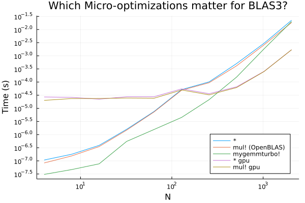
When we get to larger matrix-matrix operations, such as 100x100 * 100x100, we can effectively write off any overheads due to memory allocations. But we definitely see that there is a potential for some fairly significant performance gains in the lower end! Notice too that these gains are realized by using the pure-Julia LoopVectorization.jl as the standard BLAS tools tend to have extra threading overhead in this region (again, not optimizing as much in this region).
If you have been riding the GPU gospel without looking into the details then this plot may be a shocker! However, GPUs are designed as dumb slow chips with many cores, and thus they are only effective on very parallel operations, such as large matrix-matrix multiplications. It is from this point that assumption (2) is derived for large network operations. But again, in the case of small networks such GPU kernels will be outperformed by well-designed CPU kernels due to the lack of parallel opportunities.
Matrix-matrix operations only occur when batching is able to be used (where each column of the B matrix in A*B is a separate batch). In many cases in scientific machine learning, such as the calculation of vector-Jacobian products in ODE adjoints, this operation is a matrix-vector multiplication. These operations are smaller and only O(n^2), and as you would guess these effects are amplified in this scenario:
using LinearAlgebra, BenchmarkTools, CUDA, LoopVectorization

function mygemmturbo!(C, A, B)
    @tturbo for m ∈ axes(A, 1), n ∈ axes(B, 2)
        Cmn = zero(eltype(C))
        for k ∈ axes(A, 2)
            Cmn += A[m, k] * B[k, n]
        end
        C[m, n] = Cmn
    end
end

function alloc_timer(n)
    A = rand(Float32,n,n)
    B = rand(Float32,n)
    C = rand(Float32,n)
    t1 = @belapsed $A * $B
    t2 = @belapsed (mul!($C,$A,$B))
    t3 = @belapsed (mygemmturbo!($C,$A,$B))
    A,B,C = (cu(A), cu(B), cu(C))
    t4 = @belapsed CUDA.@sync($A * $B)
    t5 = @belapsed CUDA.@sync(mul!($C,$A,$B))
    t1,t2,t3,t4,t5
end
ns = 2 .^ (2:11)
res = [alloc_timer(n) for n in ns]
alloc      = [t[1] for t in res]
noalloc    = [t[2] for t in res]
noalloclv  = [t[3] for t in res]
allocgpu   = [t[4] for t in res]
noallocgpu = [t[5] for t in res]

using Plots
plot(ns, alloc, label="* (OpenBLAS)", xscale=:log10, yscale=:log10, legend=:bottomright,
    title="Which Micro-optimizations matter for BLAS2?",
    yticks=10.0 .^ (-8:0.5:2),
    ylabel="Time (s)", xlabel="N",)
plot!(ns,noalloc,label="mul! (OpenBLAS)")
plot!(ns,noalloclv,label="mygemvturbo!")
plot!(ns,allocgpu,label="* gpu")
plot!(ns,noallocgpu,label="mul! gpu")
savefig("microopts_blas2.png")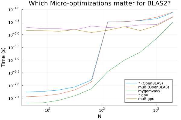
And remember, the basic operations of a neural network are sigma.(W*x .+ b), and thus there's also an O(n) element-wise operation. As you would guess, this operation becomes more significant as n gets smaller while requiring even more consideration for memory operations.
using LinearAlgebra, BenchmarkTools, CUDA, LoopVectorization

function mybroadcastturbo!(C, A, B)
    @tturbo for k ∈ axes(A, 2)
        C[k] += A[k] * B[k]
    end
end

function alloc_timer(n)
    A = rand(Float32,n,n)
    B = rand(Float32,n,n)
    C = rand(Float32,n,n)
    t1 = @belapsed $A .* $B
    t2 = @belapsed ($C .= $A .* $B)
    t3 = @belapsed (mybroadcastturbo!($C, $A, $B))
    A,B,C = (cu(A), cu(B), cu(C))
    t4 = @belapsed CUDA.@sync($A .* $B)
    t5 = @belapsed CUDA.@sync($C .= $A .* $B)
    t1,t2,t3,t4,t5
end
ns = 2 .^ (2:11)
res = [alloc_timer(n) for n in ns]
alloc      = [t[1] for t in res]
noalloc    = [t[2] for t in res]
noalloclv  = [t[3] for t in res]
allocgpu   = [t[4] for t in res]
noallocgpu = [t[5] for t in res]

using Plots
plot(ns,alloc,label="=",xscale=:log10,yscale=:log10,legend=:bottomright,
     title="Which Micro-optimizations matter for BLAS1?",
     ylabel = "Time (s)", xlabel = "N",
     yticks = 10.0 .^ (-8:0.5:2),)
plot!(ns,noalloc,label=".=")
plot!(ns, noalloc, label="mybroadcastturbo!")
plot!(ns,allocgpu,label="= gpu")
plot!(ns,noallocgpu,label=".= gpu")
savefig("microopts_blas1.png")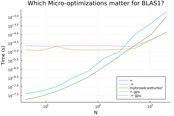
This already highly motivates a project focused on the performance for this case, but assumptions (3) and (4) point us to additionally look at the implementation of the backpropagation. The trade-off between different machine learning libraries' approaches to automatic differentiation has already been discussed at length, but what the general discussions can miss is the extra opportunities afforded when really specializing on a domain. Take for example the use-case inside of neural ordinary differential equations (neural ODEs) and ODE adjoints. As mentioned above, in this use case the backwards pass is applied immediately after the forward pass. Thus, while a handwritten adjoint to a neural network layer can look like:
ZygoteRules.@adjoint function (f::FastDense)(x,p)
  W = ...
  b = ...
  r = W*x .+ b
  y = f.σ.(r)
  function FastDense_adjoint(v)
    σbar = ForwardDiff.derivative.(f.σ,r)
    zbar = v .* σbar
    Wbar = zbar * x'
    bbar = zbar
    xbar = W' * zbar
    nothing,xbar,vcat(vec(Wbar),bbar)
  end
  y,FastDense_adjoint
end
for sigma.(W*x .+ b) to calculate J'v, you can greatly optimize this if you know that the backwards pass will immediately precede the forward pass. Specifically, there's no need to generate closures to store values since there no indeterminate future where the gradient might be needed, instead you can immediately proceed to calculate it. And, if you're only applying it to a vector of known size v, then this operation can be done without allocating by mutating a cache vector. Lastly, if we know we're only going to use the derivative w.r.t. x (xbar), then we can eliminate many calculations. Look at the simplified version:
r = W*x .+ b
y = σ.(r)
σbar = derivative.(σ,r)
zbar = v .* σbar
Wbar = zbar * x'
bbar = zbar
xbar = W' * zbar
and now cached:
mul!(cache,W,x)
cache .= σ.(cache .+ b)
cache .= derivative.(σ,cache)
cache .= v .* cache
mul!(xbar,W',cache)
or in other words, we can write this as a mutating operation with a single cache vector: vjp!(xbar,W,b,σ,v,cache). All of the overheads of any automatic differentiation or mutations? Gone.
Of course, building this up for anything other than the simplest case takes a much larger effort. In comes SimpleChains.jl.
SimpleChains.jl: An Optimized Machine Learning Library for SciML Use Cases
SimpleChains.jl is the solution to this problem. SimpleChains.jl is a small machine learning framework optimized for quickly fitting small models on the CPU. Early development favored a design that would:
Allow us to achieve good performance, ideally approaching the CPU's potential peak FLOPs.
Focus on small size meant we could largely forgo large kernel optimizations (such as cache tiling) in the early stages of development.
Have an API where vectors of parameters (and their gradients) are first class, rather than having parameters live with the layers, to make it easier to work with various optimizers or solvers that expect contiguous vectors (such as BFGS).
Be written in "pure Julia" for ease of development and optimization; while making heavy use of LoopVectorization.jl, SimpleChains.jl does not rely on any BLAS or NN libraries. It is a long term aim to extend this loop-compiler approach to optimization to also producing pullbacks automatically, without requiring them to be handwritten. However, the compiler-focused approach is already levered for ease of implementation: while we still have to hand-write gradients, we do not need to hand-optimize them.
SimpleChains.jl in Action: 30x-ing PyTorch in Tiny Example
Note: All of the code shown uses SimpleChains v0.2.2. For updates, see the package's documentation.
Let's first try a tiny example, where we map a 2x2 matrix to its matrix exponential; our training and test data:
function f(x)
  N = Base.isqrt(length(x))
  A = reshape(view(x, 1:N*N), (N,N))
  expA = exp(A)
  vec(expA)
end

T = Float32;
D = 2 # 2x2 matrices
X = randn(T, D*D, 10_000); # random input matrices
Y = reduce(hcat, map(f, eachcol(X))); # `mapreduce` is not optimized for `hcat`, but `reduce` is

Xtest = randn(T, D*D, 10_000);
Ytest = reduce(hcat, map(f, eachcol(Xtest)));
To fit this, we define the following model:
using SimpleChains
mlpd = SimpleChain(
  static(4),
  TurboDense(tanh, 32),
  TurboDense(tanh, 16),
  TurboDense(identity, 4)
)
The first layer maps the 4-dimensional input to 32 dimensions with a dense (linear) layer, applies the non-linear tanh activation. The second layer maps these 32 outputs to 16 dimensions with another dense layer, and again applies elementwise tanh, before the final layer dense layer maps these to a 4 dimensional result, which we could reshape into a 2x2 matrix, hopefully approximately equaling the exponential.
We can fit this matrix as follows:
@time p = SimpleChains.init_params(mlpd);
G = SimpleChains.alloc_threaded_grad(mlpd);

mlpdloss = SimpleChains.add_loss(mlpd, SquaredLoss(Y));
mlpdtest = SimpleChains.add_loss(mlpd, SquaredLoss(Ytest));

report = let mtrain = mlpdloss, X=X, Xtest=Xtest, mtest = mlpdtest
  p -> begin
    let train = mlpdloss(X, p), test = mlpdtest(Xtest, p)
      @info "Loss:" train test
    end
  end
end

report(p)
for _ in 1:3
  @time SimpleChains.train_unbatched!(
    G, p, mlpdloss, X, SimpleChains.ADAM(), 10_000
  );
  report(p)
end
On an Intel i9 10980XE, an 18-core system featuring AVX512 with two 512-bit fma units/core, this produces
julia> report(p)
┌ Info: Loss:
│   train = 13.402281f0
└   test = 14.104155f0

julia> for _ in 1:3
         # fit with ADAM for 10_000 epochs
         @time SimpleChains.train_unbatched!(
           G, p, mlpdloss, X, SimpleChains.ADAM(), 10_000
         );
         report(p)
       end
  4.851989 seconds (13.06 M allocations: 687.553 MiB, 10.57% gc time, 89.65% compilation time)
┌ Info: Loss:
│   train = 0.015274665f0
└   test = 0.14084631f0
  0.416341 seconds
┌ Info: Loss:
│   train = 0.0027618674f0
└   test = 0.09321652f0
  0.412371 seconds
┌ Info: Loss:
│   train = 0.0016900344f0
└   test = 0.08270371f0
This was run in a fresh session, so that the first run of train_unbatched includes compile time. Once it has compiled, each further batch of 10_000 epochs takes just over 0.41 seconds, or about 41 microseconds/epoch.
We also have a PyTorch model here for fitting this, which produces:
Initial Train Loss: 7.4430
Initial Test Loss: 7.3570
Took: 15.28 seconds
Train Loss: 0.0051
Test Loss: 0.0421
Took: 15.22 seconds
Train Loss: 0.0015
Test Loss: 0.0255
Took: 15.25 seconds
Train Loss: 0.0008
Test Loss: 0.0213
Taking over 35x longer, at about 1.5 ms, per epoch.
Trying on an AMD EPYC 7513, 32-Core CPU featuring AVX2:
julia> report(p)
┌ Info: Loss:
│   train = 11.945223f0
└   test = 12.403147f0

julia> for _ in 1:3
         @time SimpleChains.train_unbatched!(
           G, p, mlpdloss, X, SimpleChains.ADAM(), 10_000
         );
         report(p)
       end
  5.214252 seconds (8.85 M allocations: 581.803 MiB, 4.73% gc time, 84.76% compilation time)
┌ Info: Loss:
│   train = 0.016855776f0
└   test = 0.06515023f0
  0.717071 seconds
┌ Info: Loss:
│   train = 0.0027835001f0
└   test = 0.036451153f0
  0.726994 seconds
┌ Info: Loss:
│   train = 0.0017783737f0
└   test = 0.02649088f0
While with the PyTorch implementation, we get:
Initial Train Loss: 6.9856
Initial Test Loss: 7.1151
Took: 69.46 seconds
Train Loss: 0.0094
Test Loss: 0.0097
Took: 73.68 seconds
Train Loss: 0.0010
Test Loss: 0.0056
Took: 68.02 seconds
Train Loss: 0.0006
Test Loss: 0.0039
SimpleChains has close to a 100x advantage on this system for this model.
Such small models were the motivation behind developing SimpleChains. But how does it fair as we increase the problem size, to models where GPUs have traditionally started outperforming CPUs?
Edit: Timings Against Jax
The author of the Jax Equinox library submitted a Jax code for benchmarking against. On a AMD Ryzen 9 5950X 16-Core Processor we saw with Jax:
Took: 14.52 seconds
Train Loss: 0.0304
Test Loss: 0.0268
Took: 14.00 seconds
Train Loss: 0.0033
Test Loss: 0.0154
Took: 13.85 seconds
Train Loss: 0.0018
Test Loss: 0.0112
vs SimpleChains.jl with 16 threads:
5.097569 seconds (14.81 M allocations: 798.000 MiB, 3.94% gc time, 73.62% compilation time)
┌ Info: Loss:
│   train = 0.022585187f0
└   test = 0.32509857f0
  1.310997 seconds
┌ Info: Loss:
│   train = 0.0038023277f0
└   test = 0.23108596f0
  1.295088 seconds
┌ Info: Loss:
│   train = 0.0023415526f0
└   test = 0.20991518f0
or 10x performance improvement, and on 36 × Intel(R) Core(TM) i9-10980XE CPU @ 3.00GHz we saw for Jax:
Initial Train Loss: 6.4232
Initial Test Loss: 6.1088
Took: 9.26 seconds
Train Loss: 0.0304
Test Loss: 0.0268
Took: 8.98 seconds
Train Loss: 0.0036
Test Loss: 0.0156
Took: 9.01 seconds
Train Loss: 0.0018
Test Loss: 0.0111
vs SimpleChains.jl:
4.810973 seconds (13.03 M allocations: 686.357 MiB, 8.25% gc time, 89.76% compilation time)
┌ Info: Loss:
│   train = 0.011851382f0
└   test = 0.017254675f0
  0.410168 seconds
┌ Info: Loss:
│   train = 0.0037487738f0
└   test = 0.009099905f0
  0.410368 seconds
┌ Info: Loss:
│   train = 0.002041543f0
└   test = 0.0065089874f0
or ~22x speedup. With an unknown 6-core CPU with unknown threads we saw Jax:
Initial Train Loss: 6.4232
Initial Test Loss: 6.1088
Took: 19.39 seconds
Train Loss: 0.0307
Test Loss: 0.0270
Took: 18.91 seconds
Train Loss: 0.0037
Test Loss: 0.0157
Took: 20.09 seconds
Train Loss: 0.0018
Test Loss: 0.0111
vs SimpleChains.jl
13.428804 seconds (17.76 M allocations: 949.815 MiB, 2.89% gc time, 100.00% compilation time)
┌ Info: Loss:
│   train = 12.414271f0
└   test = 12.085746f0
 17.685621 seconds (14.99 M allocations: 808.462 MiB, 4.02% gc time, 48.56% compilation time)
┌ Info: Loss:
│   train = 0.034923762f0
└   test = 0.052024134f0
  9.208631 seconds (19 allocations: 608 bytes)
┌ Info: Loss:
│   train = 0.0045825513f0
└   test = 0.03521506f0
  9.258355 seconds (30 allocations: 960 bytes)
┌ Info: Loss:
│   train = 0.0026099205f0
└   test = 0.023117168f0
Thus against Jax we saw a 2x-22x, with increasing performance improvements based on the availability of threads and the existence of AVX512. More details can be found at this link, and we invite others to benchmark the libraries in more detail and share the results.
SimpleChains.jl in Action: 5x-ing PyTorch in Small Examples
Let's test MNIST with LeNet5. Note that this example will be a very conservative estimate of speed because, as a more traditional machine learning use case, batching can be used to make use of matrix-matrix multiplications instead of the even smaller matrix-vector kernels. That said, even in this case we'll be able to see a substantial performance benefit because of the semi-small network sizes.
The following is the Julia code using SimpleChains.jl for the training:
using SimpleChains, MLDatasets

lenet = SimpleChain(
  (static(28), static(28), static(1)),
  SimpleChains.Conv(SimpleChains.relu, (5, 5), 6),
  SimpleChains.MaxPool(2, 2),
  SimpleChains.Conv(SimpleChains.relu, (5, 5), 16),
  SimpleChains.MaxPool(2, 2),
  Flatten(3),
  TurboDense(SimpleChains.relu, 120),
  TurboDense(SimpleChains.relu, 84),
  TurboDense(identity, 10),
)

# 3d and 0-indexed
xtrain3, ytrain0 = MLDatasets.MNIST.traindata(Float32);
xtest3, ytest0 = MLDatasets.MNIST.testdata(Float32);

xtrain4 = reshape(xtrain3, 28, 28, 1, :);
xtest4 = reshape(xtest3, 28, 28, 1, :);

ytrain1 = UInt32.(ytrain0 .+ 1);
ytest1 = UInt32.(ytest0 .+ 1);

lenetloss = SimpleChains.add_loss(lenet, LogitCrossEntropyLoss(ytrain1));

# initialize parameters
@time p = SimpleChains.init_params(lenet);

# initialize a gradient buffer matrix; number of columns places an upper bound
# on the number of threads used.
G = similar(p, length(p), min(Threads.nthreads(), (Sys.CPU_THREADS ÷ ((Sys.ARCH === :x86_64) + 1))));

# train
@time SimpleChains.train_batched!(G, p, lenetloss, xtrain4, SimpleChains.ADAM(3e-4), 10);

SimpleChains.accuracy_and_loss(lenetloss, xtrain4, p)
SimpleChains.accuracy_and_loss(lenetloss, xtest4, ytest1, p)
# train without additional memory allocations
@time SimpleChains.train_batched!(G, p, lenetloss, xtrain4, SimpleChains.ADAM(3e-4), 10);
# assess training and test loss
SimpleChains.accuracy_and_loss(lenetloss, xtrain4, p)
SimpleChains.accuracy_and_loss(lenetloss, xtest4, ytest1, p)
PyTorch
Before we show the results, let's look at the competition. Here's two runs of 10 epochs using PyTorch following this script on an A100 GPU using a batch size of 2048:
A100:
Took: 17.66
Accuracy: 0.9491
Took: 17.62
Accuracy: 0.9692
Trying a V100:
Took: 16.29
Accuracy: 0.9560
Took: 15.94
Accuracy: 0.9749
This problem is far too small to saturate the GPU, even with such a large batch size. Time is dominated by moving batches from the CPU to the GPU. Unfortunately, as the batch sizes get larger, we need more epochs to reach the same accuracy, so we can hit a limit in terms of maximizing accuracy/time.
PyTorch using an AMD EPYC 7513 32-Core Processor:
Took: 14.86
Accuracy: 0.9626
Took: 15.09
Accuracy: 0.9783
PyTorch using an Intel i9 10980XE 18-Core Processor:
Took: 11.24
Accuracy: 0.9759
Took: 10.78
Accuracy: 0.9841
Flux.jl
The standard machine learning library in Julia, Flux.jl was benchmarked using this script with an A100 GPU. How fast was that?
julia> @time train!(model, train_loader)
 74.678251 seconds (195.36 M allocations: 12.035 GiB, 4.28% gc time, 77.57% compilation time)

julia> eval_loss_accuracy(train_loader, model, device),
       eval_loss_accuracy(test_loader, model, device)
((loss = 0.1579f0, acc = 95.3583), (loss = 0.1495f0, acc = 95.54))

julia> @time train!(model, train_loader)
  1.676934 seconds (1.04 M allocations: 1.840 GiB, 5.64% gc time, 0.63% compilation time)

julia> eval_loss_accuracy(train_loader, model, device),
       eval_loss_accuracy(test_loader, model, device)
((loss = 0.0819f0, acc = 97.4967), (loss = 0.076f0, acc = 97.6))
Flux on a V100 GPU:
julia> @time train!(model, train_loader)
 75.266441 seconds (195.52 M allocations: 12.046 GiB, 4.02% gc time, 74.83% compilation time)

julia> eval_loss_accuracy(train_loader, model, device),
       eval_loss_accuracy(test_loader, model, device)
((loss = 0.1441f0, acc = 95.7883), (loss = 0.1325f0, acc = 96.04))

julia> @time train!(model, train_loader)
  2.309766 seconds (1.06 M allocations: 1.841 GiB, 2.87% gc time)

julia> eval_loss_accuracy(train_loader, model, device),
       eval_loss_accuracy(test_loader, model, device)
((loss = 0.0798f0, acc = 97.5867), (loss = 0.0745f0, acc = 97.53))
Flux on an AMD EPYC 7513 32-Core Processor:
julia> @time train!(model, train_loader)
110.816088 seconds (70.82 M allocations: 67.300 GiB, 4.46% gc time, 29.13% compilation time)

julia> eval_loss_accuracy(train_loader, model, device),
       eval_loss_accuracy(test_loader, model, device)
((acc = 93.8667, loss = 0.213f0), (acc = 94.26, loss = 0.1928f0))

julia> @time train!(model, train_loader)
 74.710972 seconds (267.64 k allocations: 62.860 GiB, 3.65% gc time)

julia> eval_loss_accuracy(train_loader, model, device),
       eval_loss_accuracy(test_loader, model, device)
((acc = 96.7117, loss = 0.1121f0), (acc = 96.92, loss = 0.0998f0))
Flux on an Intel i9 10980XE 18-Core Processor:
julia> @time train!(model, train_loader)
 72.472941 seconds (97.92 M allocations: 67.853 GiB, 3.51% gc time, 38.08% compilation time)

julia> eval_loss_accuracy(train_loader, model, device),
       eval_loss_accuracy(test_loader, model, device)
((acc = 95.56, loss = 0.1502f0), (acc = 95.9, loss = 0.1353f0))

julia> @time train!(model, train_loader)
 45.083632 seconds (348.19 k allocations: 62.864 GiB, 2.77% gc time)

julia> eval_loss_accuracy(train_loader, model, device),
       eval_loss_accuracy(test_loader, model, device)
((acc = 97.5417, loss = 0.082f0), (acc = 97.74, loss = 0.0716f0))
How long did SimpleChains.jl take?
SimpleChains on an AMD EPYC 7513 32-Core Processor:
#Compile
julia> @time SimpleChains.train_batched!(G, p, lenetloss, xtrain4, SimpleChains.ADAM(3e-4), 10);
 34.410432 seconds (55.84 M allocations: 5.920 GiB, 3.79% gc time, 85.95% compilation time)

julia> SimpleChains.error_mean_and_loss(lenetloss, xtrain4, p)
(0.972, 0.093898475f0)

julia> SimpleChains.error_mean_and_loss(lenetloss, xtest4, ytest1, p)
(0.9744, 0.08624289f0)

julia> @time SimpleChains.train_batched!(G, p, lenetloss, xtrain4, SimpleChains.ADAM(3e-4), 10);
  3.083624 seconds

julia> SimpleChains.error_mean_and_loss(lenetloss, xtrain4, p)
(0.9835666666666667, 0.056287352f0)

julia> SimpleChains.error_mean_and_loss(lenetloss, xtest4, ytest1, p)
(0.9831, 0.053463124f0)
SimpleChains on an Intel i9 10980XE 18-Core Processor:
#Compile
julia> @time SimpleChains.train_batched!(G, p, lenetloss, xtrain4, SimpleChains.ADAM(3e-4), 10);
 35.578124 seconds (86.34 M allocations: 5.554 GiB, 3.94% gc time, 95.48% compilation time)

julia> SimpleChains.accuracy_and_loss(lenetloss, xtrain4, p)
(0.9697833333333333, 0.10566422f0)

julia> SimpleChains.accuracy_and_loss(lenetloss, xtest4, ytest1, p)
(0.9703, 0.095336154f0)

julia> # train without additional memory allocations
       @time SimpleChains.train_batched!(G, p, lenetloss, xtrain4, SimpleChains.ADAM(3e-4), 10);
  1.241958 seconds

julia> # assess training and test loss
       SimpleChains.accuracy_and_loss(lenetloss, xtrain4, p)
(0.9801333333333333, 0.06850684f0)

julia> SimpleChains.accuracy_and_loss(lenetloss, xtest4, ytest1, p)
(0.9792, 0.06557372f0)

julia> # train without additional memory allocations
       @time SimpleChains.train_batched!(G, p, lenetloss, xtrain4, SimpleChains.ADAM(3e-4), 10);
  1.230244 seconds

julia> # assess training and test loss
       SimpleChains.accuracy_and_loss(lenetloss, xtrain4, p)
(0.9851666666666666, 0.051207382f0)

julia> SimpleChains.accuracy_and_loss(lenetloss, xtest4, ytest1, p)
(0.982, 0.05452118f0)
SimpleChains on an Intel i7 1165G7 4-Core Processor (thin and light laptop CPU):
#Compile
julia> @time SimpleChains.train_batched!(G, p, lenetloss, xtrain, SimpleChains.ADAM(3e-4), 10);
 41.053800 seconds (104.10 M allocations: 5.263 GiB, 2.83% gc time, 77.62% compilation time)

julia> SimpleChains.accuracy_and_loss(lenetloss, xtrain, p),
       SimpleChains.accuracy_and_loss(lenetloss, xtest, ytest, p)
((0.9491333333333334, 0.16993132f0), (0.9508, 0.15890576f0))

julia> @time SimpleChains.train_batched!(G, p, lenetloss, xtrain, SimpleChains.ADAM(3e-4), 10);
  5.320512 seconds

julia> SimpleChains.accuracy_and_loss(lenetloss, xtrain, p),
       SimpleChains.accuracy_and_loss(lenetloss, xtest, ytest, p)
((0.9700833333333333, 0.10100537f0), (0.9689, 0.09761506f0))
Note that smaller batch sizes improve accuracy per epoch, and batch sizes were set to be proportional to the number of threads.
Benchmark Summary
Latency before the first epoch begins training is problematic, but SimpleChains.jl is fast once compiled. Post-compilation, the 10980XE was competitive with Flux using an A100 GPU, and about 35% faster than the V100. The 1165G7, a laptop CPU featuring AVX512, was competitive, handily trouncing any of the competing machine learning libraries when they were run on far beefier CPUs, and even beat PyTorch on both the V100 and A100. Again, we stress that this test case followed the more typical machine learning uses and thus was able to use batching to even make GPUs viable: for many use cases of SimpleChains.jl this is not the case and thus the difference is even larger.
However, it seems likely that the PyTorch script was not well optimized for GPUs; we are less familiar with PyTorch and would welcome PRs improving it. That said, the script is taken from a real-world user out in the wild, and thus this should demonstrate what one would expect to see from a user that is not digging into internals and hyper-optimizing. Nothing out of the ordinary was done with the Julia scripts: these were all "by the book" implementations. Though of course, the SimpleChains.jl's simplest code is specifically optimized for this "by the book" use case.
Conclusion
There are many things that can make a library achieve high-performance, and nothing is as essential as knowing how it will be used. While the big machine learning frameworks have done extremely well focusing on the top-notch performance for 99.9% of their users, one can still completely outclass them when focusing on some of the 0.1% of applications which fall outside of what they have been targeting. This is the advantage of composability and flexibility: a language that allows you to easily build a machine learning framework is also a language which allows you to build alternative frameworks which are optimized for alternative people. SimpleChains.jl will not be useful to everybody, but it will be extremely useful to those who need it.